When I first heard about inferential statistics I was amazed by that topic, How can we take conclusions about the population with just samples of it? In some way it sounds like magic.

Then someone taught me about the Central Limit Theorem and how to compare means with the t-test, but at that time I didn’t fully understood those concepts, and I realized that I just learnt how to solve problems and exercises about it.

I think it’s important to understand the Why’s and the intuition behind the theory before learning the mechanics of solving exercises about them. Now tools like Python facilitates us a lot to do that, that’s the purpose of this article. We are going to use Python to illustrate the first steps towards inferential statistics, with key concepts like Central Limit Theorem or the t-tests. As I usually say: When I code it, then I understand it.

Central Limit Theorem (CLT)

CLT states that if we have a population of some variable and take m samples of n-size, and we calculate some parameter in each sample (for example mean, median, standard deviation, etc), the distribution of that m parameters will be normal as n increases, and its variance will decrease also as n increases (distribution curve will narrow). This is true even if the original population doesn’t follow a normal distribution.

As said before, I think the best way to understand CLT is to practice with some data and obtaining the expected results. We are going to use the CLT with 3 distributions computing the mean, the median and the standard deviation.

• Uniform distribution
• Normal distribution
• Binomial distribution

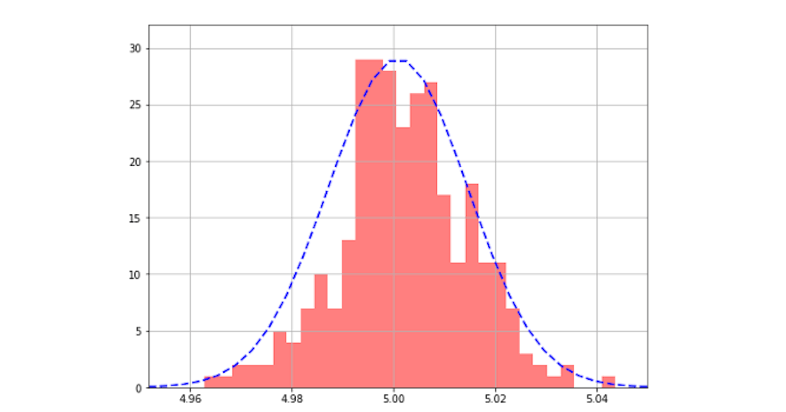
“Checking” Central Limit Theorem by plotting histograms and distribution curves increasing n (sample-sizes)

Now we are going to “check” the CLT by plotting histograms of sample parameters and show how they change if we increase n (sample-size). We’ll also plot the associated normal curve, and for that we’ll need to know the “standard error”.

It’s important to say that CLT is usually applied for the mean, but actually, as we’ll see, we can apply it for any parameter (median, variances, standard deviation…). This is relevant because, for example, sometimes the median tells us much more than the mean.

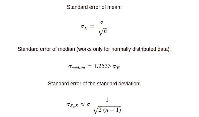
Standard Error (SE)

What is the Standard Error? It’s the standard deviation of the sampling distribution. It decreases as n (sample size) increases. Each parameter will have associated a different standard error formula. Next we show the SE expression for the SE mean, SE median, SE std.

We can “prove” this is true using the previous function. We’ll compute “manually” the standard deviation and compare it to the formula value, they should be similar.

As we can see, results are similar:

{
    "binomialdist_example (mean, n=200)": {
        "computed_se": 0.0504901583850754,
        "formula_se": 0.05815619602703747
    },
    "normaldist_example (median, n=200)": {
        "computed_se": 0.004247561325654817,
        "formula_se": 0.004343732383749954
    },
    "uniformdist_example (std, n=200)": {
        "computed_se": 0.013055146058296654,
        "formula_se": 0.02204320895687334
    }
}

Now we are going to build a function to plot histograms and distribution curves as n (sample size) increases:

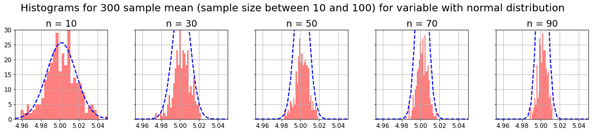
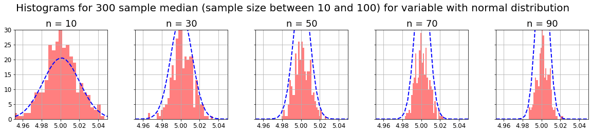
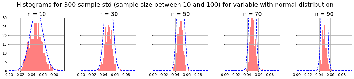
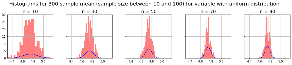
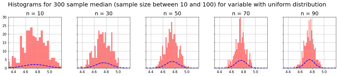
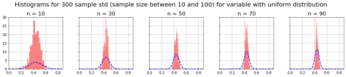
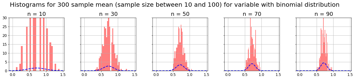
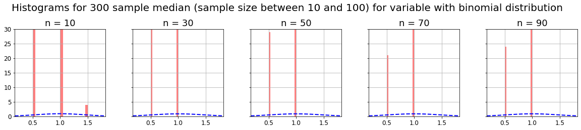
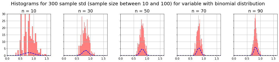
As we can see, as the CLT theorem states, with any kind of distribution, if we take m samples of n-size, and compute some parameter on them (for example mean, median or standard deviation), the distribution of that m parameters will be normal, and its variance will decrease as n increases (distribution curve will narrow).

Understanding t-test

Once we have a notion about what CLT is about, now we can apply this knowledge to understand the t-test. T-test is used normally for the following cases:

One-sample t-test

We want to check if the population mean is equal or different from the sample mean. Here we are using directly CLT theorem with this t statistic (We assume s≈σ because we don’t know the population variance): $$ t = \frac{\overline{x}-\mu}{{\frac{s}{\sqrt{n}}}} $$

Two-sample t-test

We want to check if given 2 samples, the population mean of them is equal or different. Assumptions:

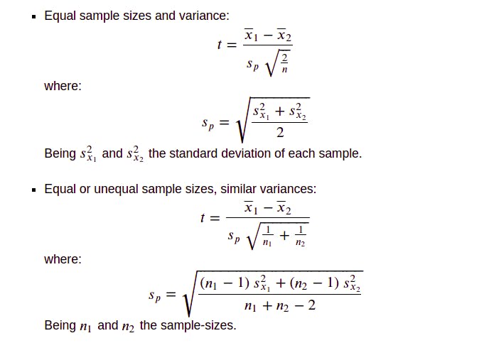
• Homogeneity of Variance:
  Population variances are assumed to be equal. I think we can have an intuition about the reason of this assumption because the t-test is actually using the CLT theorem to compare 2 means. We have to apply the proper “standard error”. The standard error depends on the sample size and population variance. Different sample sizes and variances will lead to different standard errors.
  We can find an “adjusted” standard error if sample sizes are different, but for different variances it’s better to apply a whole different test (Welch test). These are the cases and its corresponding t-values with their proper standard errors:

• Sample independence:
  It means that there are 2 different groups, that it’s not the same group that has been measured twice. If the samples are paired (dependent) t-statistic is very similar to the “One sample test” one, but our variable is the difference between samples.

$$ t = \frac{\overline{d}-\mu_d}{{\frac{s_d}{\sqrt{n}}}} $$

Where: \(\overline{d}\) is the sample mean difference.

Note: In all t-tests (1 or 2 sample test) we assume population follows a normal distribution, but as we have seen, CLT theorem states that as n increases, the sample mean (or other parameters) will follow a normal distribution.

---

Next we are going to do some examples for each test mentioned above, and we will also check that the t-statistics are correct plotting the histogram and the distribution curve (as done before with CLT).

One-sample test examples:

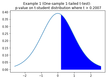
Example 1

One-sample one-tailed t-test

We have the potato yield from 12 different farms. We know that the standard potato yield for the given variety is 𝜇=20. x = [21.5, 24.5, 18.5, 17.2, 14.5, 23.2, 22.1, 20.5, 19.4, 18.1, 24.1, 18.5] Test if the potato yield from these farms is significantly better than the standard yield.

We found there is a 42% chance that 𝜇=x̄, based on our sample and it’s mean and standard deviation. So we can’t reject H0, we can’t conclude that 𝜇<x̄.

Example 2

One-sample two-tailed test

1 sample is extracted from normal-distributed population. The sample mean is x̄ = 50 and standard deviation 𝑠=5. There are 30 observations. Considering the following hypothesis:
H0: 𝜇=48
H1: 𝜇≠48
With significance of 5%, can we reject H0?

5% of significance means 2,5% per tail, as we can see in the following picture:

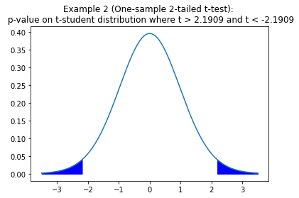
We can reject H0 with 5% of significance, meaning that is very likely that 𝜇≠48.

---

Two-sample test examples:

As said before, we want to check if given 2 samples, the population mean of them is equal or different. Here we’re going to check that the following t-statistic is correct by plotting histograms for the general case: “Equal or unequal sample sizes, similar variances”. After that we’ll do an example exercise for each case.

In order to do this check we’ll tweak “plot_histograms_sample_parameter” function, generating m samples of the difference between their sample means (with different n size). Better than describing it with words, it’s easy to understand reading code:

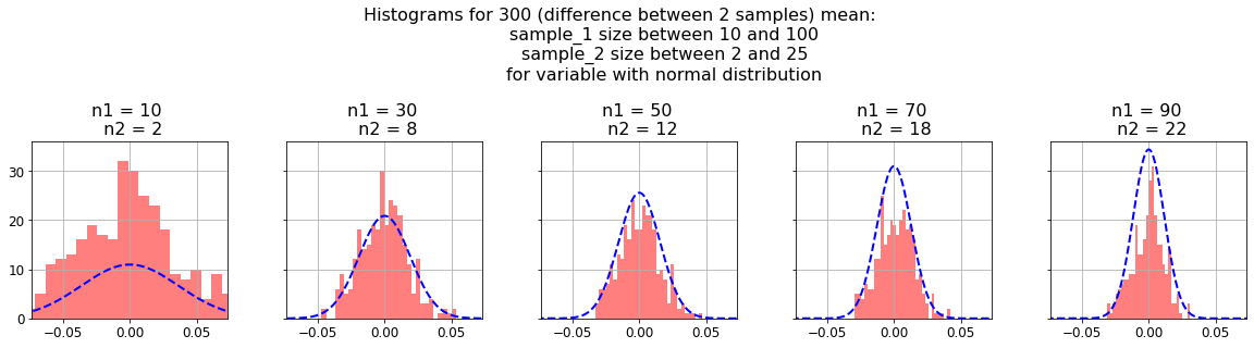
As we can see, the blue normal curves fit well in the histograms, it means that our t-statistic is correct.

Example 3

Two-sample independent t-test with different sample sizes:

We can measure person’s fitness by measuring body fat percentage. The normal range for men is 15–20%, and the normal range for women is 20–25% body fat. We have 2 sample data from a group of men and women. The following dictionary shows the data.

example3_data = {
    "men": [13.3, 6.0, 20.0, 8.0, 14.0, 19.0, 
            18.0, 25.0, 16.0, 24.0, 15.0, 1.0, 15.0],
    "women": [22.0, 16.0, 21.7, 21.0, 30.0,
             26.0, 12.0, 23.2, 28.0, 23.0]
}

Using t-test we want to know if there is difference significance between the population mean of men and women group. These will be our hypothesis.

H0: 𝜇_men = 𝜇_women
H1: 𝜇_men ≠ 𝜇_women

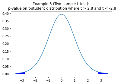
We can reject H0 with 5% of significance, meaning that is very likely that 𝜇_men ≠ 𝜇_women.

Example 4

Two-sample paired t-test:

A study was conducted to investigate the effectiveness of hypnotism in reducing pain. Results are shown in the following dataframe. The “before” value is matched to an “after” value. Are the sensory measurements, on average, lower after hypnotism? Test at 5% significance level.

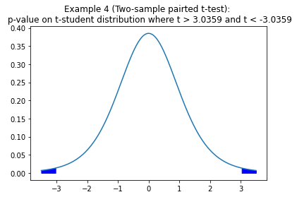
As we see, we can reject HO with a p-value of 0.009478. So, based on our data, it’s very likely that hypnotism is reducing pain.

---

Hope this article helped to understand inferential statistic key concepts as Central Limit Theorem and how t-test work, gaining confidence when applying them. Here you can find the full Jupyter Notebook used for writing this story.

---

[1]: Ahn S., Fessler, J. (2003). Standard Errors of Mean, Variance, and Standard Deviation Estimators. The University of Michigan.

[2] machinelearningplus.com. One Sample T Test — Clearly Explained with Examples | ML+. (2020, October 8). machinelearningplus.com/statistics/one-samp..

[3] bookdown.org. Practice 13 Conducting t-tests for Matched or Paired Samples in R. Retrieved April 9, 2022 from bookdown.org/logan_kelly/r_practice/p13.html

[4] jmp.com. The Two-Sample t-test. Retrieved April 9, 2022 from jmp.com/en_ch/statistics-knowledge-portal/t..