Regression is one of the most important statistical technique ever, almost every data analysis uses this method in some way. In a descriptive way, regression is used to see correlations in the data, but correlation doesn't imply always causality, as we can see in this web.

In this article we are going to use a dataset of employees as an example to find insights and relations between variables using regression, and to interpret the result reports.

Linear regression

Each employee's address is described as latitude and longitude, so we could check if there is a correlation between these variables and the employee wage. It's important to note that is fictional data (employees live in the middle of pacific ocean 🌎😂).

As we can see in the following graphs both variables seem to be correlated with wage.

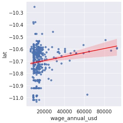
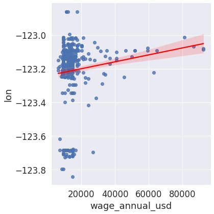
• As latitude and longitude increase (north-east direction), wages grow
• As wages grow, seems they prefer to live in the north-east of the city

But... Is there causality? If yes, which is the dependent and the independent variable? In other words, which variable is the causal of the other? This answer is not always easy to find but in this example we can infer the company is located in a city where better neighborhoods are in the north-east. So, as employees earn more, they prefer to move to the north-east of city. Wage is the independent variable and latitude and longitude, dependents.

Definitions:

• Causal Effects for variable X: Changes in outcomes due to changes in X, holding all the rest of the variables constant. Later we are going to make a model to predict employees' wage based on several variables like gender, age, location, etc. We can say there is a causal effect on wage due to gender if, holding the rest of variables constant, and changing the gender, causes a change in wage.
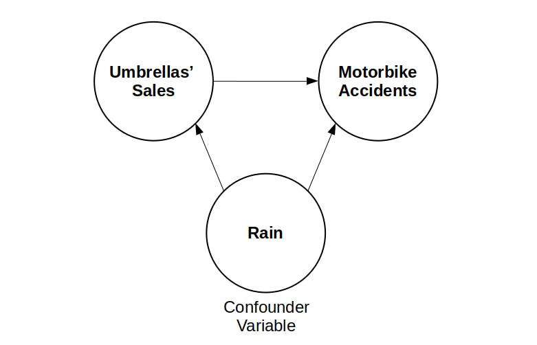
• Confounding variable: Variable that influences both the dependent variable and the independent variable, causing a spurious association. Imagine we find that motorbike accidents are highly correlated with the sale of umbrellas. As umbrellas' sales go up, motorbike accidents increase. We could think that umbrellas' sales are the causal of motorbike accidents, but what really happens is that rain is affecting both variables (umbrellas and accidents).

Interpreting linear regression output

Now we are going to interpret the linear regression report, taking as an example the wage-latitude regression. This is the equation for simple linear regression: $$ y = \alpha + \beta \ x $$

Next table shows the regression report:

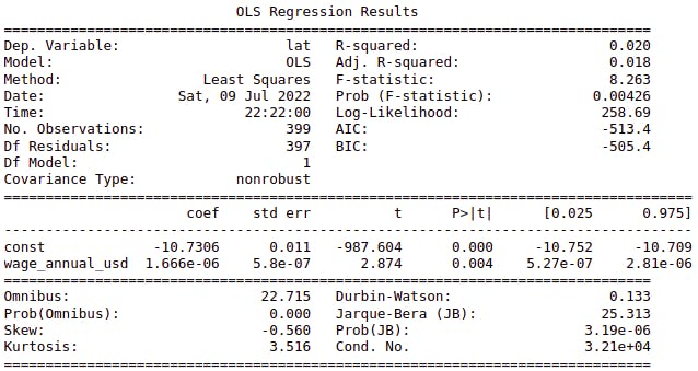
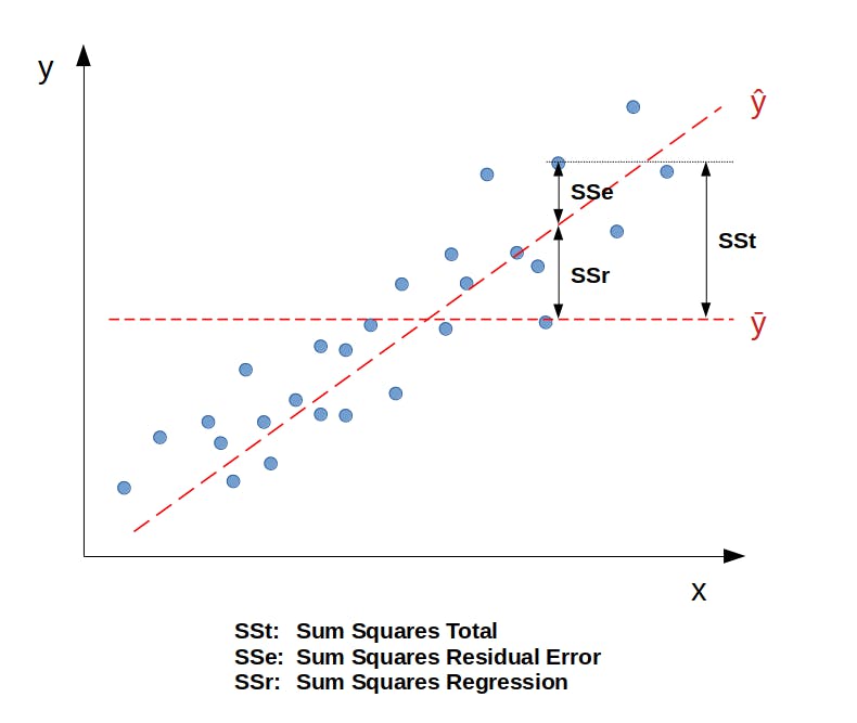
• R-squared: This number is the % of the variance explained by the model. In our case it's just 2%, a very low number, but still positive (better than an horizontal line with the mean value). $$ R^2 = 1 - \frac{\text{unexplained variation}}{\text{total variation}} = 1 - \frac{SS_r}{SS_t} = 1- \frac{\sum_i y_i-\hat{y}}{\sum_i y_i-\overline{y}} $$

• Adjusted R-squared: R-squared comes with an inherent problem, the fact that if we add any independent variable to the regression (multilinear regression), even if the variable doesn't have any relation with the dependent one, R-squared will increase or keep equal. The adjusted R-square "fixes" that problem. Adjusted R-squared is always less than or equal to R-squared. $$ R^2_{\text{adjusted}} = 1- \frac{(1 - R^2) \ (n-1)}{n-k-1} $$ Where \(n\) is the number of points in our data sample, and \(k\) the number of independent variables.

• F-statistic: This test is used to see if we can reject the following null hypothesis: $$ H_0: \beta = 0 $$ $$ H_1: \beta \neq 0 $$ If we can't reject H0 means that our regression is useless, because our coefficient is not statistically significant. As we can see in the output for the wage-latitude regression, p-value is less than 5%, then we can reject H0, meaning that our slope coefficient is statistically significant.

• Log-likelihood, AIC, BIC: Without getting too into the math, the log-likelihood (\(l\)) measures how strong a model is in fitting the data. The more parameters we add, log-likelihood will increase, but we don't want our model to over-fit, that's why we add the number of parameters (\(k\)) into the equation. $$ \text{AIC} = 2 \ k - 2 \ l $$ $$ \text{BIC} = \ln{(n)} \ k - 2 \ l \ $$ When comparing models, we should pick the one with the lowest AIC and BIC (low number of parameters and highest log-likelihood). AIC and BIC differ in the first coefficient, BIC is the one to use if the models we're comparing have different number of samples, because it normalizes it with the term (\(\ln{n}\))

• Variables section: This is maybe the most important part in the regression outpu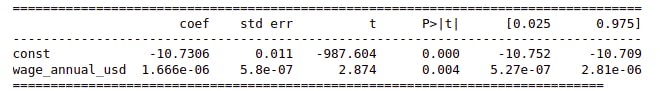t. It means that our equation would look like follows: $$ \text{latitude} = -10,73 + 1.67 \times 10^{-6} \ \text{wage} $$ The rest of the table (standard_error, t, p_value, confidence_interval), is showing us in reality one piece of information in different ways, and that's the coefficient statistical significance. The constant term (const) doesn't tell us too much (theoretically would be the wage for latitude = 0), but has to be there to build our line equation. In our example, wage term has p_value = 0,4%, < 5%, so we can consider it's statistical significant.

Multilinear regression

Usually reality is too complex to explain one term with just one parameter, that's the reason why we want to add more variables in our regression: $$ y = \beta_0 + \beta_1 \ x_1 + \beta_2 \ x_2+ \beta_3 \ x_3 + \text{...} + \beta_i \ x_i $$

Following our employees' example dataset, now we're going to make a model to predict the wage based on latitude and longitude (the other way around than before). Later we'll make another model with more parameters and check if our regression improves.

This is our regression outcome:

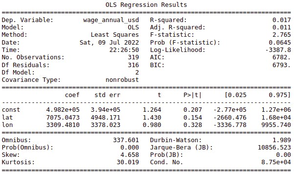
As we can see, this regression doesn't have much value for the following reasons:

• F-statistic p_value is greater than 5%, meaning that we can't reject the null hypothesis: $$ H_0: \beta_1 = \beta_2 = 0 $$
• All coefficients p_value are also greater than 5%.
• R-squared is less than 2%.

Now we're going to try to improve the model adding the following variables:

• Gender
• Age
• Nationality
• Civil status
• Contract type (fixed or indefinite term)
• Management level (top-level, middle-level, low-level, laborer)

As you can see, almost all of these variables are categorical (except age), then, in order to apply regression, we have to convert them into dummy variables. We can do these easily with pandas as follows:

df = pd.get_dummies(df, columns=['gender', 'nationality_group', 'management_level', 'contract_type'], drop_first=True)

We use drop_first because in categorical variables, if we know (n-1), we can infer the missing one (example: contract_type_indefinite_term = 0 means fixed_term contract).

Next regression output is shown:

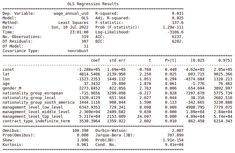
This model is much better than the one before:

• F-statistic p_value < 5%
• Many of the regression-parameters are statistically significant. Higher t-values correspond to management_level, meaning that that variable is clearly affecting wage.
• R-squared is explaining 83% of variance (highly improvement from the previous model).
• AIC and BIC are lower than the previous model.

Now we can measure model's accuracy through the following concepts:

• MAE: Mean Absolute Error = 3.912 USD $$ \text{MAE} = \frac{1}{n} \sum_{i=1}^{n} |\text{actual_values} - \text{predicted_values}| $$
• RMSE: Root Mean Squared Error = 6.578 USD $$ \text{RMSE} = \sqrt{ \frac{1}{n} \sum_{i=1}^{n} (\text{actual_values} - \text{predicted_values})^2} $$

Logistic regression

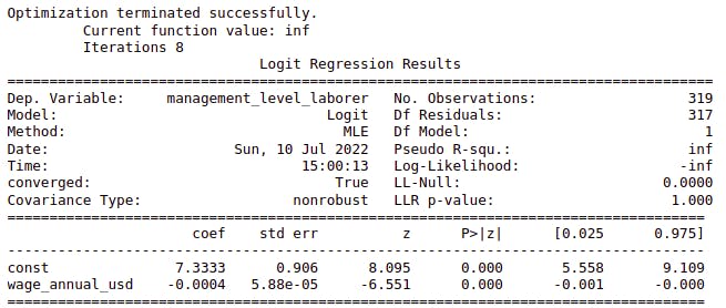
We use logistic regression when the dependent variable is categorical. For example, using our employees' dataset, let's say we want to predict whether an employee is a laborer or not, based on wage. $$ p(x) = \frac{1}{1+e^{-(\beta_0+\beta_1 \ x)}} $$

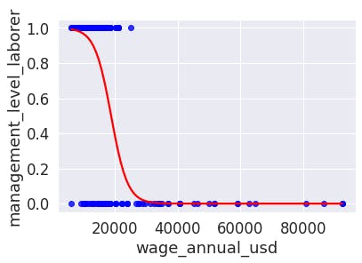Next table is the logistic regression output:

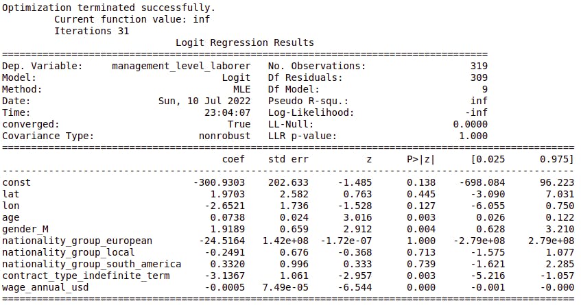
Multinomial logistic regression

The same way we can make a multilinear regression, we can build a multilogistic regression, using more than 1 independent variable. Following same example as before, we can try to predict whether an employee is a laborer or not, not only with wage, but also with other parameters like age, gender, nationality, etc.

$$ p(x) = \frac{1}{1+e^{-(\beta_0+\beta_1 \ x_1 +\beta_2 \ x_2+ \text{...} + \beta_m \ x_m)}} $$

---

Here you can find the Jupyter notebook and the dataset. used to write this article.

Thank you for reading!